Tutorial for Testing the MCAR Case

In this tutorial, we show how to test the MCAR case using the Little and the PKLM tests.

First, import some libraries

from matplotlib import pyplot as plt

import numpy as np
import pandas as pd
from scipy.stats import norm
from sklearn import utils as sku

from qolmat.analysis.holes_characterization import LittleTest, PKLMTest
from qolmat.benchmark.missing_patterns import UniformHoleGenerator

plt.rcParams.update({"font.size": 12})
seed = 1234
rng = sku.check_random_state(seed)

Generating random data

data = rng.multivariate_normal(mean=[0, 0], cov=[[1, 0], [0, 1]], size=200)
df = pd.DataFrame(data=data, columns=["Column 1", "Column 2"])

q975 = norm.ppf(0.975)

1. Testing the MCAR case with the Little’s test and the PKLM test.

The Little’s test

First, we need to introduce the concept of a missing pattern. A missing pattern, also called a pattern, is the structure of observed and missing values in a dataset. For example, in a dataset with two columns, the possible patterns are: (0, 0), (1, 0), (0, 1), (1, 1). The value 1 (0) indicates that the column value is missing (observed).

The null hypothesis, H0, is: “The means of observations within each pattern are similar.”.

The PKLM test

The test compares distributions of different missing patterns.

The null hypothesis, H0, is: “Distributions within each pattern are similar.”. We choose to use the classical threshold of 5%. If the test p-value is below this threshold, we reject the null hypothesis. This notebook shows how the Little and PKLM tests perform on a simplistic case and their limitations. We instantiate a test object with a random state for reproducibility.

little_test_mcar = LittleTest(random_state=rng)
pklm_test_mcar = PKLMTest(random_state=rng)

Case 1: MCAR holes (True negative)

hole_gen = UniformHoleGenerator(
    n_splits=1, random_state=rng, subset=["Column 2"], ratio_masked=0.2
)
df_mask = hole_gen.generate_mask(df)
df_nan = df.where(~df_mask, np.nan)

has_nan = df_mask.any(axis=1)
df_observed = df.loc[~has_nan]
df_hidden = df.loc[has_nan]

plt.scatter(
    df_observed["Column 1"],
    df_observed[["Column 2"]],
    label="Fully observed values",
)
plt.scatter(
    df_hidden[["Column 1"]],
    df_hidden[["Column 2"]],
    label="Values with missing C2",
)

plt.legend(
    loc="lower left",
    fontsize=8,
)
plt.xlabel("Column 1")
plt.ylabel("Column 2")
plt.title("Case 1: MCAR data")
plt.grid()
plt.show()

little_result = little_test_mcar.test(df_nan)
pklm_result = pklm_test_mcar.test(df_nan)
print(f"The p-value of the Little's test is: {little_result:.2%}")
print(f"The p-value of the PKLM test is: {pklm_result:.2%}")

The p-value of the Little's test is: 4.62%
The p-value of the PKLM test is: 45.16%

The two p-values are larger than 0.05, therefore we don’t reject the H0 MCAR assumption. In this case, this is a true negative.

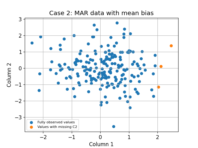
Case 2: MAR holes with mean bias (True positive)

df_mask = pd.DataFrame(
    {"Column 1": False, "Column 2": df["Column 1"] > q975}, index=df.index
)

df_nan = df.where(~df_mask, np.nan)

has_nan = df_mask.any(axis=1)
df_observed = df.loc[~has_nan]
df_hidden = df.loc[has_nan]

plt.scatter(
    df_observed["Column 1"],
    df_observed[["Column 2"]],
    label="Fully observed values",
)
plt.scatter(
    df_hidden[["Column 1"]],
    df_hidden[["Column 2"]],
    label="Values with missing C2",
)

plt.legend(
    loc="lower left",
    fontsize=8,
)
plt.xlabel("Column 1")
plt.ylabel("Column 2")
plt.title("Case 2: MAR data with mean bias")
plt.grid()
plt.show()

little_result = little_test_mcar.test(df_nan)
pklm_result = pklm_test_mcar.test(df_nan)
print(f"The p-value of the Little's test is: {little_result:.2%}")
print(f"The p-value of the PKLM test is: {pklm_result:.2%}")

The p-value of the Little's test is: 0.01%
The p-value of the PKLM test is: 3.23%

The two p-values are smaller than 0.05, therefore we reject the H0 MCAR assumption. In this case, this is a true positive.

Case 3: MAR holes with any mean bias (False negative)

The specific case is designed to emphasize the Little’s test limits. In this case, we generate holes when the absolute value of the first feature is high. This missingness mechanism is clearly MAR but the means between missing patterns is not statistically different.

df_mask = pd.DataFrame(
    {"Column 1": False, "Column 2": df["Column 1"].abs() > q975},
    index=df.index,
)

df_nan = df.where(~df_mask, np.nan)

has_nan = df_mask.any(axis=1)
df_observed = df.loc[~has_nan]
df_hidden = df.loc[has_nan]

plt.scatter(
    df_observed["Column 1"],
    df_observed[["Column 2"]],
    label="Fully observed values",
)
plt.scatter(
    df_hidden[["Column 1"]],
    df_hidden[["Column 2"]],
    label="Values with missing C2",
)

plt.legend(
    loc="lower left",
    fontsize=8,
)
plt.xlabel("Column 1")
plt.ylabel("Column 2")
plt.title("Case 3: MAR data without any mean bias")
plt.grid()
plt.show()

little_result = little_test_mcar.test(df_nan)
pklm_result = pklm_test_mcar.test(df_nan)
print(f"The p-value of the Little's test is: {little_result:.2%}")
print(f"The p-value of the PKLM test is: {pklm_result:.2%}")

The p-value of the Little's test is: 19.18%
The p-value of the PKLM test is: 3.23%

The Little’s p-value is larger than 0.05, therefore, using this test we don’t reject the H0 MCAR assumption. In this case, this is a false negative since the missingness mechanism is MAR.

However the PKLM test p-value is smaller than 0.05 therefore we reject the H0 MCAR assumption. In this case, this is a true negative.

Limitations and conclusion

In this tutorial, we can see that Little’s test fails to detect covariance heterogeneity between patterns.

We also note that Little’s test does not handle categorical data or temporally correlated data.

This is why we have implemented the PKLM test, which makes up for the shortcomings of the Little test. We present this test in more detail in the next section.

2. The PKLM test

The PKLM test is very powerful for several reasons. Firstly, it covers the concerns that Little’s test may have (covariance heterogeneity). Secondly, it is currently the only MCAR test applicable to mixed data. Finally, it proposes a concept of partial p-value which enables us to carry out a variable-by-variable diagnosis to identify the potential causes of a MAR mechanism.

There is a parameter in the paper called size.res.set. The authors of the paper recommend setting this parameter to 2. We have chosen to follow this advice and not leave the possibility of increasing this parameter. The results are satisfactory and the code is simpler.

It does have one disadvantage, however: its calculation time.

Calculation time

n_rows	n_cols	Calculation time
200	2	2”12
500	2	2”24
500	4	2”18
1000	4	2”48
1000	6	2”42
10000	6	20”54
10000	10	14”48
100000	10	4’51”
100000	15	3’06”

2.1 Parameters and Hyperparameters

To use the PKLM test properly, it may be necessary to understand the use of hyper-parameters.

• nb_projections: Number of projections on which the test statistic is calculated. This parameter has the greatest influence on test calculation time. Its default value nb_projections=100.

• nb_permutation : Number of permutations of the projected targets. The higher is better. This parameter has little impact on calculation time. Its default value nb_permutation=30.

• nb_trees_per_proj : The number of subtrees in each random forest fitted. In order to estimate the Kullback-Leibler divergence, we need to obtain probabilities of belonging to certain missing patterns. Random Forests are used to estimate these probabilities. This hyperparameter has a significant impact on test calculation time. Its default value is nb_trees_per_proj=200

• compute_partial_p_values: Boolean that indicates if you want to compute the partial p-values. Those partial p-values could help the user to identify the variables responsible for the MAR missing-data mechanism. Please see the section 2.3 for examples. Its default value is compute_partial_p_values=False.

• encoder: Scikit-Learn encoder to encode non-numerical values. Its default value encoder=sklearn.preprocessing.OneHotEncoder()

• random_state: Controls the randomness. Pass an int for reproducible output across multiple function calls. Its default value random_state=None

2.2 Application on mixed data types

As we have seen, Little’s test only applies to quantitative data. In real life, however, it is common to have to deal with mixed data. Here’s an example of how to use the PKLM test on a dataset with mixed data types.

n_rows = 100

col1 = rng.rand(n_rows) * 100
col2 = rng.randint(1, 100, n_rows)
col3 = rng.choice([True, False], n_rows)
modalities = ["A", "B", "C", "D"]
col4 = rng.choice(modalities, n_rows)

df = pd.DataFrame({"Numeric1": col1, "Numeric2": col2, "Boolean": col3, "Object": col4})

hole_gen = UniformHoleGenerator(
    n_splits=1,
    ratio_masked=0.2,
    subset=["Numeric1", "Numeric2", "Boolean", "Object"],
    random_state=rng,
)
df_mask = hole_gen.generate_mask(df)
df_nan = df.where(~df_mask, np.nan)
df_nan.dtypes

Numeric1    float64
Numeric2    float64
Boolean      object
Object       object
dtype: object

pklm_result = pklm_test_mcar.test(df_nan)
print(f"The p-value of the PKLM test is: {pklm_result:.2%}")

The p-value of the PKLM test is: 29.03%

To perform the PKLM test over mixed data types, non-numerical features need to be encoded. The default encoder in the PKLMTest class is the default OneHotEncoder from scikit-learn. If you wish to use an encoder adapted to your data, you can perform this encoding step beforehand, and then use the PKLM test. Currently, we do not support the following types :

• datetimes

• timedeltas

• Pandas datetimetz

2.3 Partial p-values

In addition, the PKLM test can be used to calculate partial p-values. There are as many partial p-values as there are columns in the input dataframe. This “partial” p-value corresponds to the effect of removing the patterns induced by variable k.

Let’s take a look at an example of how to use this feature

data = rng.multivariate_normal(
    mean=[0, 0, 0, 0], cov=[[1, 0, 0, 0], [0, 1, 0, 0], [0, 0, 1, 0], [0, 0, 0, 1]], size=400
)
df = pd.DataFrame(data=data, columns=["Column 1", "Column 2", "Column 3", "Column 4"])

df_mask = pd.DataFrame(
    {
        "Column 1": False,
        "Column 2": df["Column 1"] > q975,
        "Column 3": False,
        "Column 4": False,
    },
    index=df.index,
)
df_nan = df.where(~df_mask, np.nan)

The missing-data mechanism is clearly MAR. Intuitively, if we remove the second column from the matrix, the missing-data mechanism is MCAR. Let’s see how the PKLM test can help us identify the variable responsible for the MAR mechanism.

pklm_test = PKLMTest(random_state=rng, compute_partial_p_values=True)
result = pklm_test.test(df_nan)
if isinstance(result, tuple):
    p_value, partial_p_values = result
else:
    p_value = result
print(f"The p-value of the PKLM test is: {p_value:.2%}")

The p-value of the PKLM test is: 3.23%

The test result confirms that we can reject the null hypothesis and therefore assume that the missing-data mechanism is MAR. Let’s now take a look at what partial p-values can tell us.

for col_index, partial_p_v in enumerate(partial_p_values):
    print(f"The partial p-value for the column index {col_index + 1} is: {partial_p_v:.2%}")

The partial p-value for the column index 1 is: 3.23%
The partial p-value for the column index 2 is: 100.00%
The partial p-value for the column index 3 is: 3.23%
The partial p-value for the column index 4 is: 3.23%

As a result, by removing the missing patterns induced by variable 2, the p-value rises above the significance threshold set beforehand. Thus in this sense, the test detects that the main culprit of the MAR mechanism lies in the second variable.