Comparison of basic imputers

In this tutorial, we show how to use the Qolmat comparator (comparator) to choose the best imputation between two of the simplest imputation methods: mean or median (ImputerSimple). The dataset used is the numerical superconduct dataset and contains information on 21263 superconductors. We generate holes uniformly at random via UniformHoleGenerator

import matplotlib
import matplotlib.pyplot as plt
import numpy as np
from sklearn import utils as sku

from qolmat.benchmark import comparator, missing_patterns
from qolmat.imputations import imputers
from qolmat.utils import data, plot

seed = 1234
rng = sku.check_random_state(seed)

1. Data

The data contains information on 21263 superconductors. Originally, the first 81 columns contain extracted features and the 82nd column contains the critical temperature which is used as the target variable. The data does not contain missing values; so for the purpose of this notebook, we corrupt the data, with the qolmat.utils.data.add_holes() function. In this way, each column has missing values.

df = data.add_holes(
    data.get_data("Superconductor"), ratio_masked=0.2, mean_size=120, random_state=rng
)

The dataset contains 82 columns. For simplicity, we only consider some.

columns = [
    "criticaltemp",
    "mean_atomic_mass",
    "mean_FusionHeat",
    "mean_ThermalConductivity",
    "mean_Valence",
]
df = df[columns]
cols_to_impute = df.columns

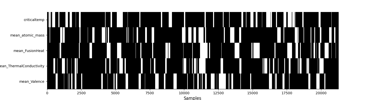
Let’s take a look at the missing data. In this plot, a white (resp. black) box represents a missing (resp. observed) value.

plt.figure(figsize=(15, 4))
plt.imshow(
    df.notna().values.T, aspect="auto", cmap="binary", interpolation="none"
)
plt.yticks(range(len(df.columns)), df.columns)
plt.xlabel("Samples", fontsize=12)
plt.grid(False)
plt.show()

2. Imputation

This part is devoted to the imputation methods. In this tutorial, we only focus on mean and median imputation. In order to use the comparator, we have to define a dictionary of imputers, a way to generate holes (additional missing values on which the imputers will be evaluated) and a list of metrics.

imputer_mean = imputers.ImputerSimple(strategy="mean")
imputer_median = imputers.ImputerSimple(strategy="median")
dict_imputers = {"mean": imputer_mean, "median": imputer_median}

metrics = ["mae", "wmape", "kl_columnwise"]

Concretely, the comparator takes as input a dataframe to impute, a proportion of nan to create, a dictionary of imputers (those previously mentioned), a list with the columns names to impute, a generator of holes specifying the type of holes to create. in this example, we have chosen the uniform hole generator. For example, by imposing that 10% of missing data be created ratio_masked=0.1 and creating missing values in columns subset=cols_to_impute:

generator_holes = missing_patterns.UniformHoleGenerator(
    n_splits=2, subset=cols_to_impute, ratio_masked=0.1, random_state=rng
)
df_mask = generator_holes.generate_mask(df)
df_mask = np.invert(df_mask).astype("int")

df_tot = df.copy()
df_tot[df.notna()] = 0
df_tot[df.isna()] = 2
df_tot += df_mask

colorsList = [(1, 0, 0), (0, 0, 0), (1, 1, 1)]
custom_cmap = matplotlib.colors.ListedColormap(colorsList)

plt.figure(figsize=(15, 4))
plt.imshow(
    df_tot.values.T, aspect="auto", cmap=custom_cmap, interpolation="none"
)
plt.yticks(range(len(df_tot.columns)), df_tot.columns)
plt.xlabel("Samples", fontsize=12)
plt.grid(False)
plt.show()

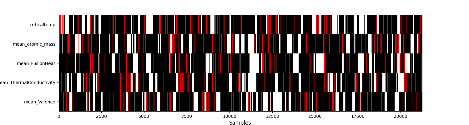
Now that we’ve seen how hole generation behaves, we can use it in the comparator.

comparison = comparator.Comparator(
    dict_imputers,
    generator_holes=generator_holes,
    metrics=metrics,
    max_evals=5,
)

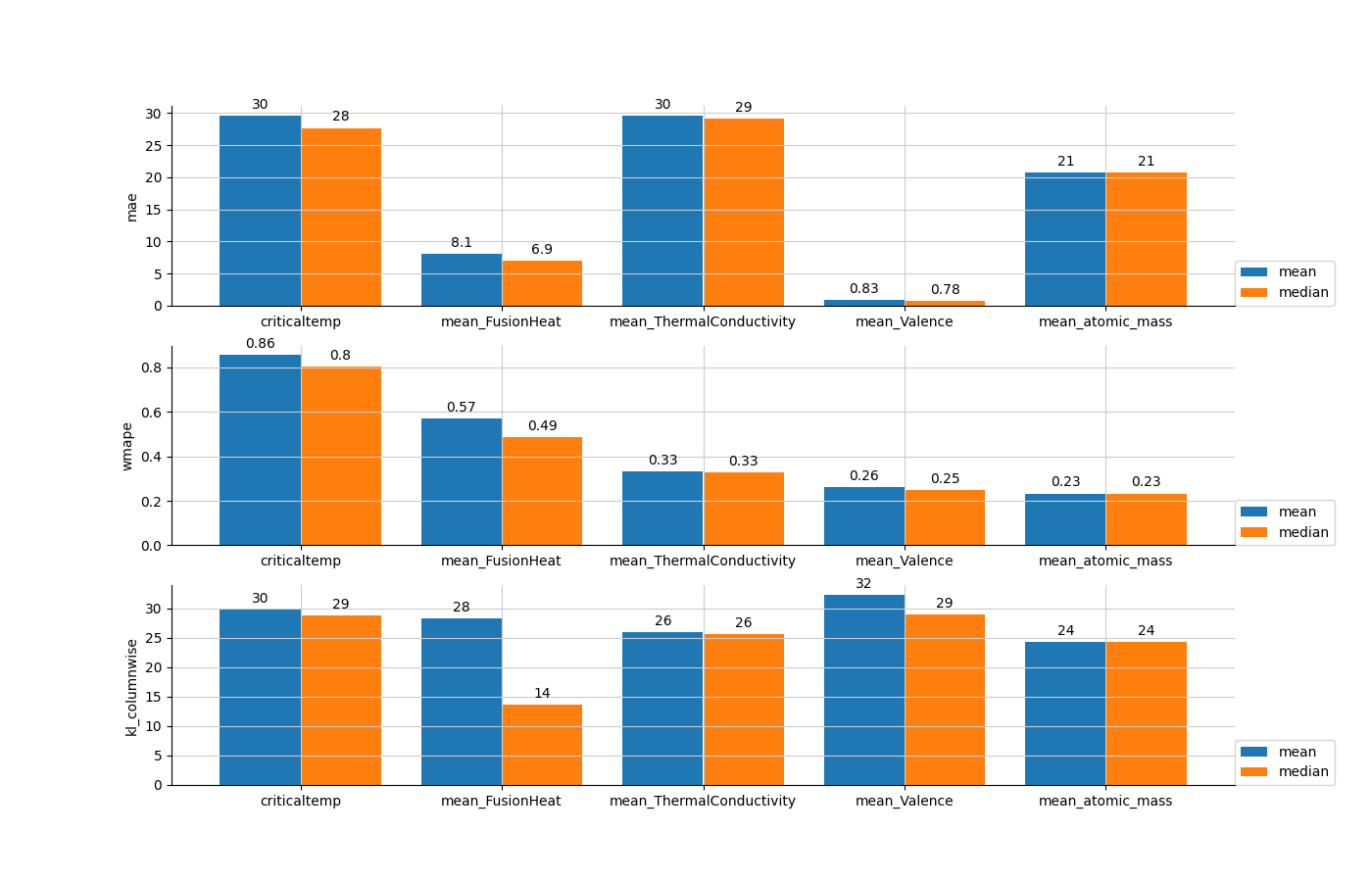
On the basis of the results, we can see that imputation by the median provides lower reconstruction errors than those obtained by imputation by the mean, except for the mean_atomic_mass with MAE.

results = comparison.compare(df)
results.style.highlight_min(color="lightsteelblue", axis=1)

		mean	median
kl_columnwise	criticaltemp	29.699655	28.770511
	mean_FusionHeat	28.283599	13.688591
	mean_ThermalConductivity	25.868046	25.545719
	mean_Valence	32.290397	28.979781
	mean_atomic_mass	24.258423	24.258423
mae	criticaltemp	29.505923	27.669155
	mean_FusionHeat	8.112540	6.944263
	mean_ThermalConductivity	29.626863	29.174941
	mean_Valence	0.825231	0.775617
	mean_atomic_mass	20.671858	20.683861
wmape	criticaltemp	0.855155	0.801891
	mean_FusionHeat	0.568664	0.486700
	mean_ThermalConductivity	0.331483	0.326426
	mean_Valence	0.262622	0.246824
	mean_atomic_mass	0.232943	0.233077

Let’s visualize this dataframe.

n_metrics = len(metrics)
fig = plt.figure(figsize=(14, 3 * n_metrics))
for i, metric in enumerate(metrics):
    fig.add_subplot(n_metrics, 1, i + 1)
    plot.multibar(results.loc[metric], decimals=2)
    plt.ylabel(metric)
plt.show()

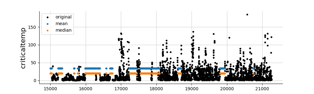
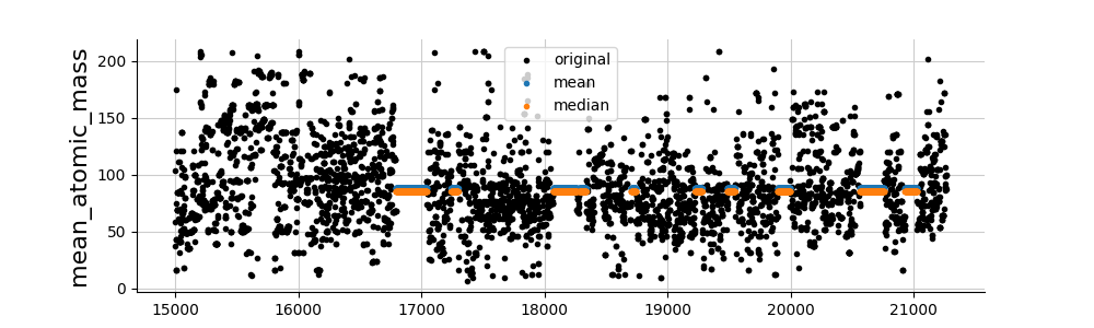
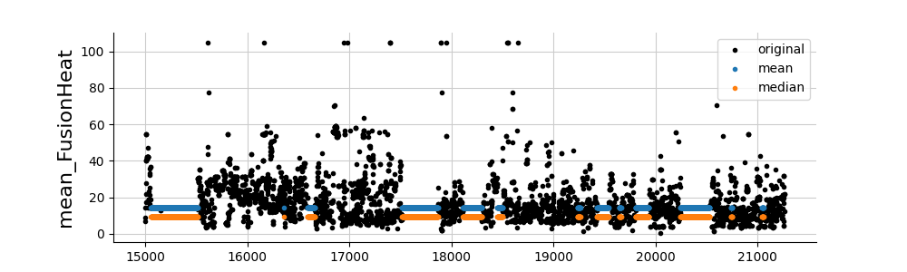
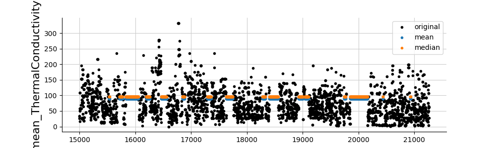
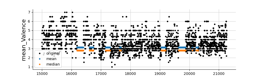
And finally, let’s take a look at the imputations. Whatever the method, we observe that the imputations are relatively poor. Other imputation methods are therefore necessary (see folder imputations).

dfs_imputed = {
    name: imp.fit_transform(df) for name, imp in dict_imputers.items()
}

for col in cols_to_impute:
    fig, ax = plt.subplots(figsize=(10, 3))
    values_orig = df[col]
    plt.plot(values_orig[15000:], ".", color="black", label="original")
    for ind, (name, model) in enumerate(list(dict_imputers.items())):
        values_imp = dfs_imputed[name][col].copy()
        values_imp[values_orig.notna()] = np.nan
        plt.plot(values_imp[15000:], ".", label=name, alpha=1)
    plt.ylabel(col, fontsize=16)
    plt.legend()
    plt.show()

• 
• 
• 
• 
•